Hey
there!
During
last months, I was thinking with my friend Javi Fajardo (see his work
here!) a little bit more about Brownian / OU process and their
applications in biology. Remember that an OU model describes a
stochastic Markov process that consist of two parts: first, a
Brownian motion (random walk) model that represents a completely
random process of variable evolution, and a second term that
represents the attraction of an optimum value of the variable. For
this, OU process can be considered as a variation of Brownian motion
model. In the last posts we were talking about these kinds of models
used to drive trait character evolution, specifically an ecological
trait, such as optimum temperature or precipitation.
My
colleague
Javi and I were talking
about the applications of this models in two dimensions, representing
for example space coordinates (latitude/longitude). They
have been used, for example, to simulate predator/prey movements,
home range movements, etc. We
developed an R function similar to the previous eMotion
function in order implement this kind of movement models: eWalk
(from
evolutiveWalk...). eWalk
is similar to other movement-simulation functions in adehabitatLT
package
(Calenge, 2006).
However, you can use eWalk
to
simulate a variety of processes as Brownian motion, OU processes or
Lèvy flights (see below).
Here
you have the (commented!)
code
to
load the function into R console:
eWalk <- function(sigma,lon,lat, generations,alpha_x,theta_x,alpha_y,theta_y, color,levy=FALSE, plot=TRUE) {
  route=data.frame(1:generations,1:generations)                             # a data.frame to store the route
  names(route)<-c("lon","lat")
  generation= generations                                               # generation counter

  while (generation > 0){                                                   # stops the simulation when generation counter is 0
    if (levy == TRUE){                                                      # only if levy=TRUE: Levy Flight!
      rndm=abs(rcauchy(1))                                                  # process to select if I should jump or not
      if (rndm > 15){                                                       # Levy jump probability threshold
        l=15                                                                # length of the jump
        x= lon + (l * (sigma * rnorm(1))) + (alpha_x * ( theta_x - lon))    # Brownian or OU process for longitude
        y= lat + (l * (sigma * rnorm(1))) + (alpha_y * ( theta_y - lat))    # Brownian or OU process for latitude
        loc=cbind(x,y)
        route[generation,]<- loc                                            # store new location
        generation= generation - 1                                        # advance to next generation
        lon<- x                                                        # go to the new position!
        lat<- y

      }
      else{                                                                 # if Levy jump is not selected, l=1 i.e. proceed with
        l=1                                                                 #normal Brownian motion or OU process
        x= lon + (l * (sigma * rnorm(1))) + (alpha_x * ( theta_x - lon))
        y= lat + (l * (sigma * rnorm(1))) + (alpha_y * ( theta_y - lat))
        loc=cbind(x,y)
        route[generation,]<- loc
        generation= generation - 1
        lon<- x
        lat<- y
      }
    }
    else{                                                                   # if levy=FALSE, l=1, only Brownian motion or OU
      l=1
      x= lon + (l * (sigma * rnorm(1))) + (alpha_x * ( theta_x - lon))
      y= lat + (l * (sigma * rnorm(1))) + (alpha_y * ( theta_y - lat))
      loc=cbind(x,y)
      route[generation,]<- loc
      generation= generation - 1
      lon<- x
      lat<- y
    }
  }

  if (plot == TRUE) {                                                       # if plot=TRUE, plto the route!
    lines(route, col= color, lwd=3)
  }
  return(route)                                                             # print the data.frame with each location during the walk!

}
>
The
needed parameters to run the function are similar to those for
eMotion,
but taking into account that now you have two variables
(latitude/longitude, for example) at the same time.
eWalk(sigma,initial_lon,initial_lat,number
of generations, lon_alpha, lon_optimum, y_alpha, y_optimum, color,
levy=FALSE, plot=TRUE)
In
addition, I have added a complement to simulate Lèvy flights, a
non-gaussian process similar to Brownian motion but allowing for
jumps during the motion. Lévy flights pattern has been found in
searching
movements of predators (Bartumeus
et al., 2005),
or have been used to simulate
punctuated equilibrium in traits
evolution (Gould and
Eldredge, 1977; Landis
et al., 2013).
To
perform Lèvy flight, eWalk selects a random number from Cauchy
distribution and if it is higher than a threshold (15 by default),
Brownian motion term is multiplied by a constant representing a jump
(also 15 by default). Although
this is not the formal expression of a Lèvy process, this is a
simple way to simulate a negative exponential rate in for the length
of each step.
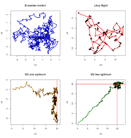
Here
you have some examples using eWalk and their code to reproduce them:
 par(mfrow=c(2,2))

a=eWalk(0.15,0,0,1000, 0, 0, 0, 0, color="blue", levy=FALSE, plot=FALSE)
plot(a,type="n", main="Brownian motion")
lines(a,lwd=3, col="blue")
points(a, cex=.3, col="black", pch=21)

a=eWalk(0.15,0,0,1000, 0, 0, 0, 0, color="red", levy=TRUE, plot=FALSE)
plot(a,type="n", main="Lêvy flight")
lines(a,lwd=3, col="red")
points(a, cex=.3, col="black", pch=21)

a=eWalk(0.15,0,0,1000, 0.01, 20, 0, 0, color="orange", levy=FALSE, plot=FALSE)
plot(a,type="n", main="OU one optimum")
lines(a,lwd=3, col="orange")
abline(v=20, col="red", lwd="2")
points(a, cex=.3, col="black", pch=21)

a=eWalk(0.15,0,0,1000, 0.01, 20, 0.01, 20, color="green", levy=FALSE, plot=FALSE)
plot(a,type="n", main="OU two optimum")
lines(a,lwd=3, col="green")
points(a, cex=.3, col="black", pch=21)
abline(v=20, col="red", lwd="2")
abline(h=20, col="red", lwd="2")
References
-Bartumeus, F., da
Luz, M. E., Viswanathan, G. M., & Catalan, J. (2005). Animal
search strategies: a quantitative random‐walk analysis. Ecology,
86(11), 3078-3087.
-Calenge, C. (2006).
The package “adehabitat” for the R software: a tool for the
analysis of space and habitat use by animals. Ecological
modelling, 197(3), 516-519.
-Gould, S. J., &
Eldredge, N. (1977). Punctuated equilibria: the tempo and mode of
evolution reconsidered. Paleobiology, 3(02), 115-151.
-Landis, M. J.,
Schraiber, J. G., & Liang, M. (2013). Phylogenetic analysis using
Lévy processes: finding jumps in the evolution of continuous traits.
Systematic biology, 62(2), 193-204.


